How to use the MATCH function Microsoft Excel
The MATCH function in Microsoft Excel is a Lookup and Reference function, and its purpose is to search for specific items in a range of cell and then returns the relative position of that item in the range. The formula for the MATCH is MATCH(lookup_ value, lookup_array[match_type]).
The syntax for the Match Function is:
- Lookup_ value: The value you want to match in the lookup_array. It is required.
- Lookup_array: The range of cells being searched. It is required.
- Match_type: Specifies how lookup_value matches with lookup_array. It is optional.
In Microsoft Excel, there are three types of match_type 1,0,-1. The “1” match_type finds the largest value that is less than or equal to the look_up value. The” 0 “ match_type finds the first value that is exactly equal to the lookup_value. The “-1 “match_type finds the smallest value that is greater than or equal to the lookup value
How to use the MATCH function in Excel
To use the MATCH function in Excel, follow the methods below:
- Launch Excel
- Create a table or use an existing table
- Enter the formula = MATCH(lookup_ value, lookup_array[match_type]) into the cell you want the result to be
- Press Enter
- See the result.
Launch Excel.
Create a table or use an existing table.

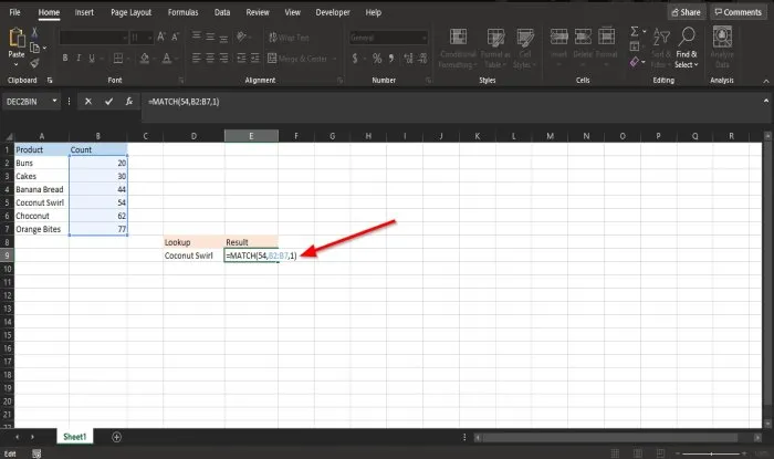
Enter the formula =MATCH (54, B2:B7,1 ) into the cell you want the result to be.
54 is the Lookup_value you want to match with the lookup array.
B2:B7 is the Lookup_array and the range of cells being searched.
1 is the Match_type, and its purpose is to specify how lookup_value matches with lookup_array.
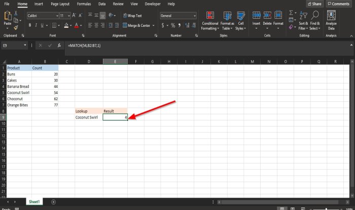
Press the Enter key to get the result
There are two other methods to use the MATCH function in Excel.
Method one is to click the fx button on the top left of the Excel worksheet.
An Insert Function dialog box will appear.
Inside the dialog box in the section, Select a Category, select Lookup and Reference from the list box.
In the section Select a Function, choose the MATCH function from the list.
Then click OK.
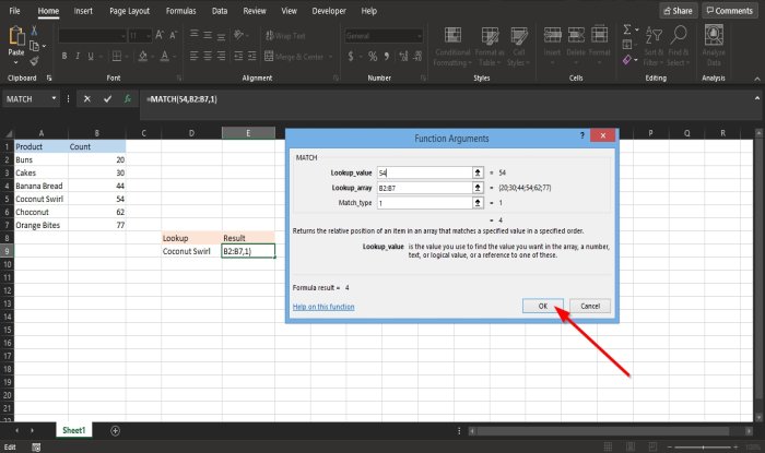
A Function Arguments dialog box will open.
In the LookUp_ value box, type 54.
In the LookUp_ array box, type B2:B7.
In the Match_type box, type 1.
Then click OK to see the result.
Method Two is to click the Formulas tab and click the Lookup and Reference button in the Function Library group.
In the drop-down menu, select the MATCH function.
A Function Arguments dialog box will appear.
Follow the steps in method one for Function Arguments.
We hope this tutorial helps you understand how to use the MATCH function in Microsoft Excel; if you have questions about the tutorial, let us know in the comments.
Read next: How to use the DEC2Bin function in Microsoft Excel to convert a decimal number to binary.


