How to apply color in alternate rows or columns in Excel

If you want to apply color in alternate rows and columns in an Excel spreadsheet, here is what you need to do. It is possible to show the desired color in every alternate row or column with the Conditional Formatting. This functionality is included in Microsoft Excel, and you can make use of it with the help of this tutorial.

Let’s assume that you are making a spreadsheet for your school or office project, and you have to colorize every alternate row or column. There are two ways to do that in Microsoft Excel. First, you can select particular rows or columns and change the background color manually. Second, you can use the Conditional Formatting functionality to apply the same in automation. Either way, the result will be the same, but the second method is more efficient and time saving for any user.

How to alternate row colors in Excel

To apply color in alternate rows or columns in Excel, follow these steps-

1. Open the spreadsheet with Excel.
2. Select the rows and columns that you want to colorize.
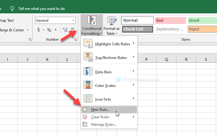
3. Click the Conditional Formatting in the Home tab.
4. Select New Rule from the list.
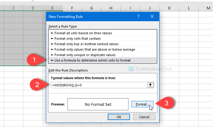
5. Select Use a formula to determine which cells to format.
6. Enter =MOD(ROW(),2)=0 or =MOD(COLUMN(),2)=0 in the Format values box.
7. Click the Format button.
8. Switch to the Fill tab.
9. Select a color that you want to use.
10. Click the OK button twice.

Let’s check out these steps in detail.

At first, open the spreadsheet with Excel. In case, you do not have the spreadsheet, create it first so that you can understand whether you want to colorize the rows or columns. Once done, use your mouse to select all the cells (rows and columns). If you’re going to apply the color scheme to the entire spreadsheet, click the arrow icon that allows you to select the spreadsheet from top to bottom.

Now make sure that you are in the Home tab. If so, click on the Conditional Formatting in the Styles section, and select the New Rule option from the list.

Following that, select the Use a formula to determine which cells to format option, and write down one of these in the Format values box-

• =MOD(ROW(),2)=0
• =MOD(COLUMN(),2)=0

The first one will colorize the desired color in alternate rows and the second one is for columns. After that, click the Format button.

Now, switch to the Fill tab, select a color that you want to use, and click on the OK button.

Then, you will have to click the OK button again to apply the change.

That’s all! Now you can see the selected color in every alternate row or column.