How to create Barcode in Excel

Here is a tutorial to generate a barcode in Microsoft Excel. You might want to generate barcodes in Excel to make a product catalog or to track stocked items in Excel or for any other reason. This guide will show you the steps you need to use to create normal and random barcodes in your Excel spreadsheets.

Although there is no native option, you can still easily create a barcode in your Excel workbooks. To do so, you just need to use a custom barcode font to generate a particular type of barcode, such as Code 39, Code 128, Universal Product Codes (UPC), International Article Number (EAN), etc. These fonts are freely available on the internet. You can simply download and install the font you want in Office and then create barcodes in Excel. Let us check out a step-by-step procedure for the same.

How to create Barcode in Excel

Here, we will generate barcodes of Code 39 type. So, we will be using a free Code 39 font to generate the barcode. However, you can pick any other barcode font based on the type and use it to create a barcode in your Excel workbook. Here are the basic steps to create a barcode in Excel:

1. Download and install Code 39 font in Office.
2. Launch Excel and create a new blank spreadsheet.
3. Create two columns with Text and Barcode names.
4. Format the cells in the Text column.
5. Enter a formula in the Barcode column.
6. Select the barcode font for the cells in the Barcode column.
7. Enter alphanumeric data in the Text column for which you want to generate a barcode.

Let us check out these barcode creation steps in detail!

Firstly, you need to install a Code 39 font in Office. You will have to download this font from the internet. There are various free font downloader websites to get this font from.

After downloading the font file, install the Code 39 font in Office. We have used a Code 39 font from here. Simply unzip the downloaded font folder, double click on the TTF font file, and then in the opened window, click on the Install button.

After installing the Code 39 font, launch the Excel application and create a new blank workbook. Now, create two columns with the names Text and Barcode.

Next, you have to format the cells in the Text column. For that, select the entire Text column and right-click on it. From the context menu, select the Format Cells option.

After that, from the Number tab, click on the Text category and press the OK button. This will basically preserve leading zeroes and also, larger numbers won’t be displayed in scientific notation.

Now, you need to enter the ="*"&A2&"*" formula in the first cell of the Barcode column. We suppose A2 is the first cell of the Text column. If it’s a different column and cell number, e.g., C2, D2, etc., you can adjust the formula accordingly. In case there is no text in the Text Column, it will display two asterisks.

You now have to copy the above formula to all the cells in the Barcode column. Just select the first cell and then drag the cursor from the bottom-right corner toward the end of the column. This will apply the entered formula to all the cells in the Barcode column.

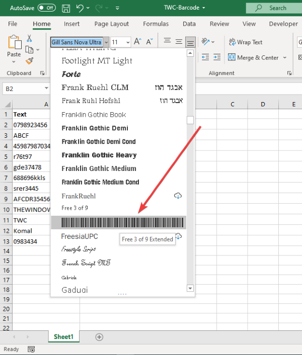
Next, select all the cells in the Barcode column and go to the Home > Font option. From here, choose the installed Code 39 font and you will see a barcode in the respective cells. Also, add the text for which you want to generate a barcode in the Text column.

As soon as you select the barcode font, you will see a barcode in the Barcode column for the text in the Text column.

How to Generate Random Barcodes in Excel

You can also generate a random barcode in Excel. This can be done using the RANDBETWEEN function. Using this function, you can generate random numbers, random strong passwords, and even random barcodes. In addition to the above-discussed steps, you can follow the below steps to create random barcodes in Excel:

After that selecting the barcode font for the Barcode column (refer to general barcode generation method above), go to the Text column. Select the entire column and right-click on it. Click on the Format Cell option and go to the Number tab and make sure it is set to General.

Now, select the first cell in the Text column. In the function bar, type the following formula: =RANDBETWEEN(X,Y). The X is the lowest value and Y is the highest value. It basically defines the range to generate a number. For example, =RANDBETWEEN(5000,11000). This will generate a random number between 5000 to 11000.

Next, copy this formula to all cells in the Text column by dragging the cursor from the first cell to the last cell. Doing so will generate random numbers in the entire Text column and you will be able to view respective random barcodes in the Barcode column.

That’s about it! Hope you find this article helpful!

Now read: How to Create a Barcode in Microsoft Word.