How to switch Rows and Columns in Excel

When creating a chart, the program figures out the correct way to organize the data; the program determines which to labels to assign to the horizontal axis and where to put the chart’s legend, but what if there is an error? For instance, you want the rows of the data displayed on the horizontal axis to be displayed on the vertical axis instead. So you can switch the rows to columns so that the data can demonstrate the way you want; this is done using the Switch Row/ Column button.

How to switch Rows and Columns in Excel

The Switch Row or Column feature allows the user to swap data over the axis; the data on the X-axis will move to the Y-axis. It’s a feature that transforms the data in the chart.

1. Launch Microsoft Excel
2. Create a chart or use an existing chart
3. Click the Chart
4. Click the Chart Design tab
5. Click the Switch Row / Column button
6. The rows are switch to column

To switch the rows and columns in an excel chart, follow the methods below.

Launch Microsoft Excel.

Create a statistical table or used an existing one.

Highlight the table.

Then go to Insert and select a Chart in the Charts group; in this tutorial, we have chosen a Bar Chart.

Once you click the Bar Chart, select the Bar Chart you want from the drop-down list.

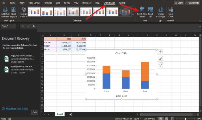
Now that the chart is created, a Chart Design tab will appear on the menu bar.

If you have an existing chart, you can also use it.

On the tab in the Data group, click the Switch Row / Column button.

The rows are switch to columns.

We hope this tutorial helps you understand how to switch rows and columns in an Excel Chart.

Read next: How to use the DVAR function in Excel.