How to write, build, and use VLOOKUP function in Excel

The VLOOKUP function in Microsoft Excel literally means vertical lookup. It’s a search function for querying values in the cell of a column. This function searches for the data relative to the entries in the first column from the left.

A vertical data search is most vital when dealing with tables with numerous columns and rows. Instead of scrolling through and analyzing hundreds of cells, Excel’s VLOOKUP function helps you find the data you’re looking for by looking up the values from top to bottom.

Create, build & use Excel’s VLOOKUP function

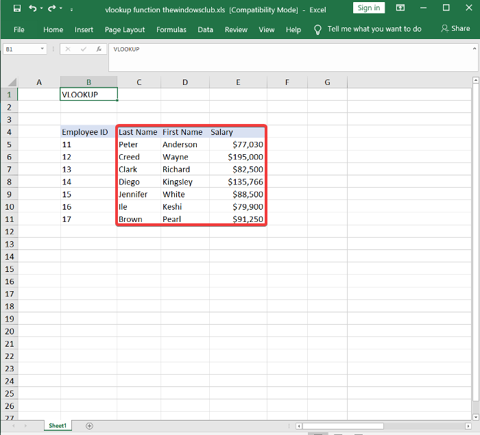
In our example, we’ll work with a VLOOKUP function that searches for information about seven employees’ salaries. This section shows you how to use the VLOOKUP function in the following ways:

1. Write the Excel VLOOKUP function.
2. Build a VLOOKUP function in Excel.

Without further ado, let’s get to it. In the first method, we’ll create the function manually. Next, we’ll use it from Excel’s inbuilt Functions Arguments wizard.

1] Write the Excel VLOOKUP function

Launch Microsoft Excel and make a column for the values that act as unique identifiers. We’ll call this the reference column.

Add some more columns to the right-hand side of the first one you created in the first step and insert values for the cells in these columns.

Click on an empty cell in the spreadsheet and type in an Employee ID from the reference column of an employee for whom you wish to search for data.

Select another empty cell on the spreadsheet in which Excel will store the formula and hence display the returned value. Here, enter the following formula:

=VLOOKUP()

On entering the above formula, Excel suggests the VLOOKUP syntax:

=VLOOKUP(vlookup_value,table_array,col_index_num,range_lookup)

Arguments or parameters

Here are what the above arguments define in the syntax:

• lookup_value: the cell with the product identifier from the reference column.
• table_array: the data range from with to search. It must contain the reference column and the column containing the value you’re looking up. In most cases, you can use the entire worksheet. You can drag your mouse over the values of the table to select a data range.
• col_index_num: the number of the column from which to look up a value. You put this in from left to right.
• range_lookup: TRUE for an approximate match, FALSE for an exact match. The value is TRUE by default, but you generally use FALSE.

With this information, we’ll now replace the parameters in the parenthesis with the information we wish to look up. For example, to return Wayne Creed‘s salary, enter the following formula:

=VLOOKUP(C14,B5:E11,6,FALSE)

On navigating away from the cell with the VLOOKUP formula, it returns the value for which you queried. If you get a #N/A error, read this Microsoft guide to learn how to correct it.

2] Build a VLOOKUP function in Excel

The first part showed you how to create a VLOOKUP function manually. If you thought the above method was easy, wait till you read this. Here, you’ll learn how to build a VLOOKUP function quickly using the user-friendly Functions Arguments wizard.

Open Microsoft Excel first, and create a reference column that will contain unique identifiers.

Next, create some more columns on the right-hand side of the reference column. Here, we’ll insert the relevant values for the items on the reference column.

Select an empty cell and type in a value from the reference cell. This is the value whose properties we’ll lookup.

Click on another empty cell. With that selected, click on the Formulas tab.

Select the Lookup & Reference tool from the Functions Library and choose VLOOKUP from the dropdown menu. This opens the Functions Arguments wizard.

Fill in the Lookup_value, Table_array, Col_index_num, and Range_lookup fields in the Functions Arguments wizard specified in the first method.

Hit the OK button when you’re done, and the VLOOKUP function will return the results from the arguments you entered.

This guide will help you if the Excel formula fails to update automatically.

Both methods will successfully query the data you need in reference to the first column. The Formulas Argument wizard makes it easy to input the variables to make the VLOOKUP function work.

This guide was based on Microsoft Excel for Windows 10.

However, the VLOOKUP function also works on the web version of Excel. You also get to use the Functions Argument wizard or create the VLOOKUP function manually on the web version.